This chapter builds on the principles presented in chapter 3. That chapter was ended with an example showing the relationship between two variables. In this chapter more predictor variables (independent variables) are added to the model. (Remember the Y'=a + bx is the model being considered.) There are no new principles added -- just complexity. In multiple there may be many independent variables and one dependent variable.
In this next section Y primed (Y'), Beta, regression line slope, and the constant are discussed. As implied in the formula Y'=a +bX these concepts are related.
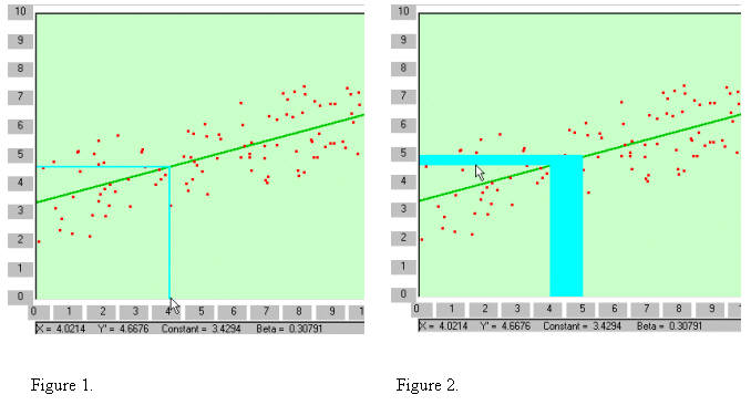
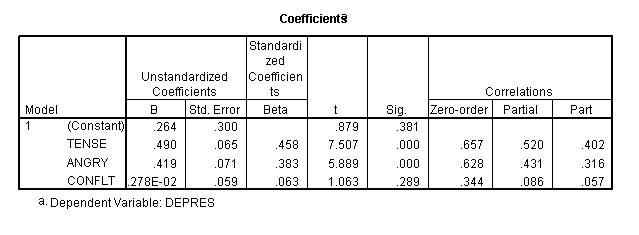
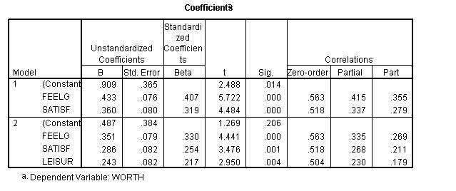
Beta is the change in Y for each unit (1) change of X. In the example above the change of X from 4 to 5 (actually 4.0214 to 5.0214) shows a change in Y as .30791. This is seen in Figure 2 by the light blue shaded area (if you are viewing in black and white it is the shaded area identified by the cursor). The vertical blue area represents 1 for X. That from 4 to 5. The left side of the blue area identifies 4 on the x-axis and when it meets the regression line a horizontal line to the y-axis is the Y value predicted by 4 on the x-axis (Y' for 4). The right side of the blue area identifies 5 on the x-axis and when it meets the regression line a horizontal line to the Y-axis is the Y value predicted by 5 on the X-axis (Y' for 5). The difference between Y' when X=4 and Y' when X=5 is beta. It is represented by the horizontal blue area.
The constant (a) is the value of Y when X is zero. It is 3.4294. It can be thought of as the origin or the regression line. Once the starting point of the regression line is identified (the constant--a) the remainder can be generated by beta. That is the slope can be determined using beta. Points are plotted according the unit changes in X. The next plot after X=0 would be when X=1. A line is drawn from X=1 up to the point on Y that is equal to the constant plus beta. That is, 3.4294 plus .30791 which is 3.73731. Next .030791 is added to 3.73731 at the X=2 position and a point identified. Once these points are drawn the regression line can be drawn through these points as indicated above.
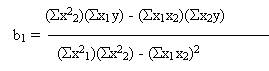
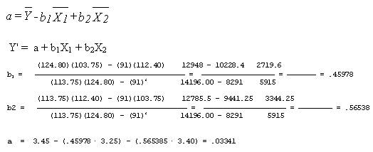
With this information a prediction can be made by using Y'. That is if X is known and one has the constant and beta then Y can be predicted using the following formula:
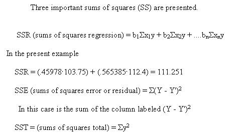
The difference between Y' and the actual score is the error in prediction. When all of the differences are squared and summed the result is the error sum of squares. The square root of the sum of squares error divided by N is the error variance.
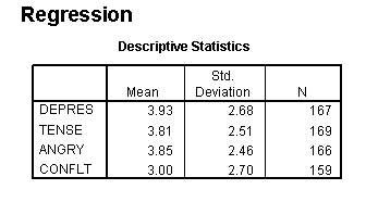
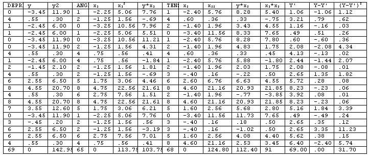
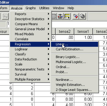
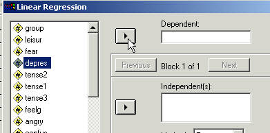
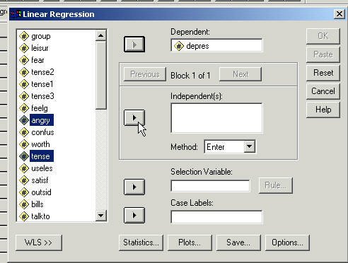
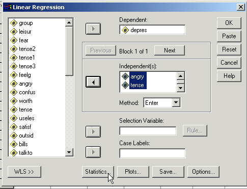
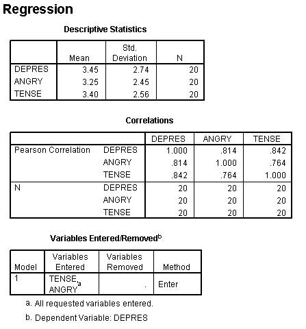
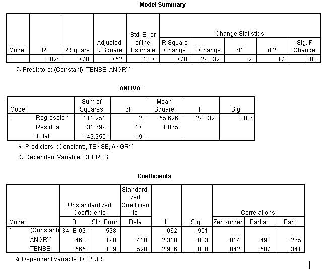
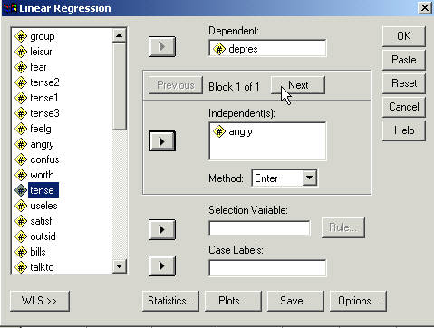
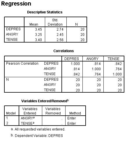
In chapter 3 the two variables DEPRES and TENSE (taken from the Psychosocial Assessment Scale) were correlated using the regression method. In this example the variable ANGRY is added to the model. The variable DEPRES will be treated as the criterion variable (dependent variable); while TENSE and ANGRY will be treated at the predictor variables (independent variables).
The following data is taken from the data found in Figure 1 in chapter.
Although all of the formulae presented in chapter 3 apply here only the extended formulae related to multiple variables.
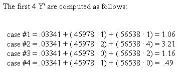
Notice that the results of these cases corresponds to the column identified as Y' (y primed) in the table above.
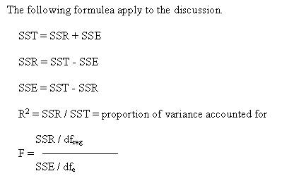
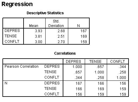
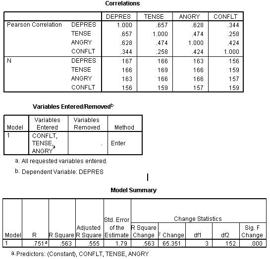
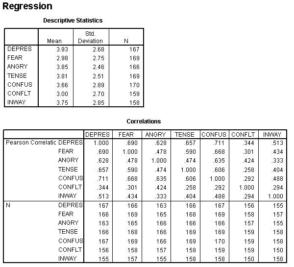
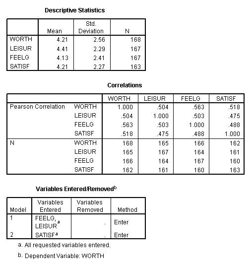
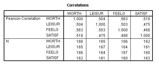
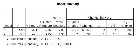
R square and consequently the amount of shared variance between two or more variables can be obtained by (1) squaring the correlation and (2) multiplying that result time 100.
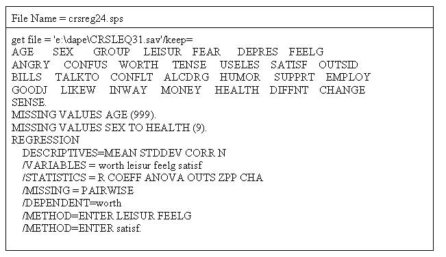
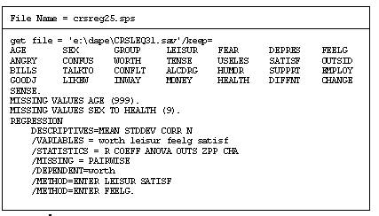
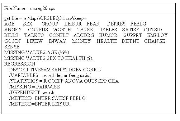
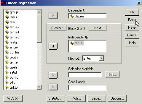
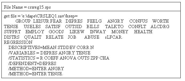
Click Paste
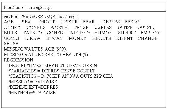
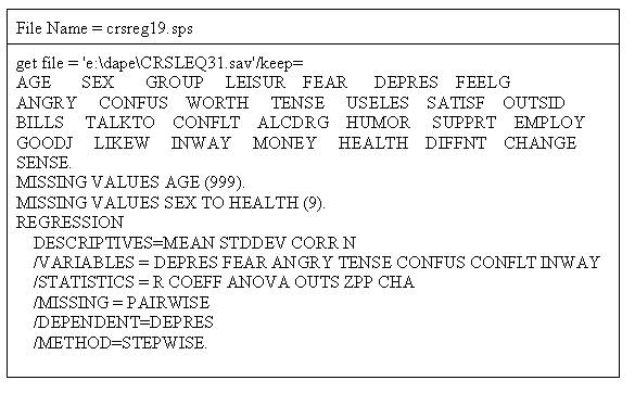
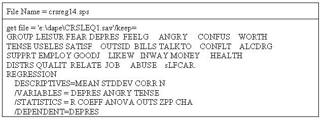
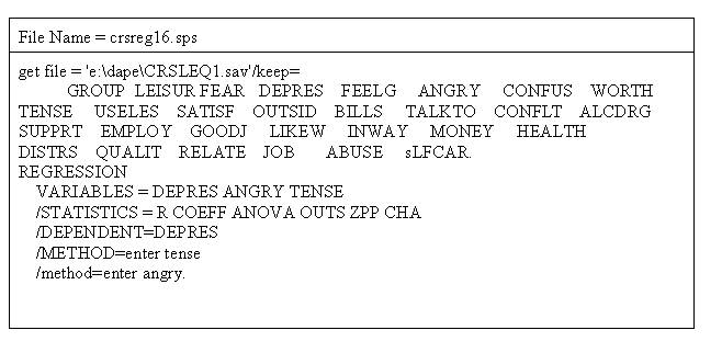
That will produce approximately the following syntax file (the "keep" command will not be there).
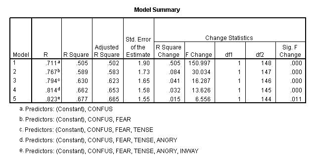
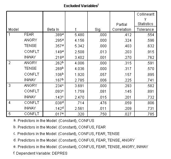
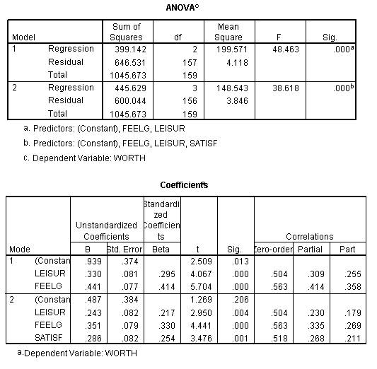
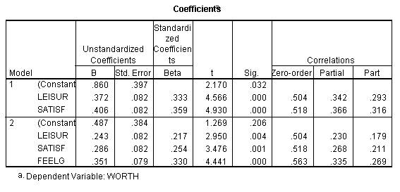
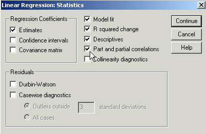
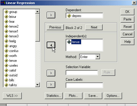
This next set of examples is designed to show (1) that you can test the contribution of each variable, (2) that you can force variables to enter the model (a new concept model) to be tested for their contribution, and (3) that the computer will select the next variable that will contribute the most to model (step wise regression).
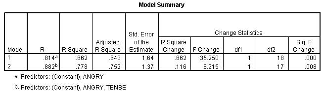
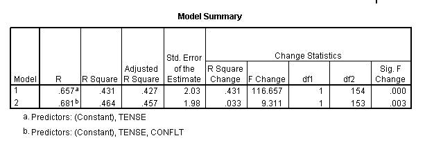
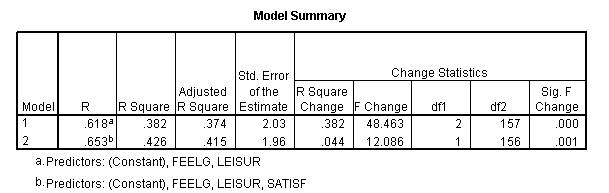
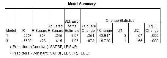
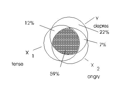
Notice that the R Square Change for variable 2 (Tense) is .116. That is the proportion of change and can be converted to percentage of variance accounted for by multiplying by 100 which makes it 11.6% when rounded becomes 12%. This variance is referred to as unique variance. It is variance of the Y variable that is shared only with Tense. Or stated differently it is variance of the Y variable that is accounted by Tense only.
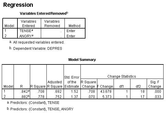
Notice that the R Square Change for variable 2 (Angry) is .070. That is the proportion of change and can be converted to percentage of variance accounted for by multiplying by 100 which makes it 7 or 7%.
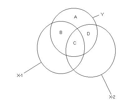
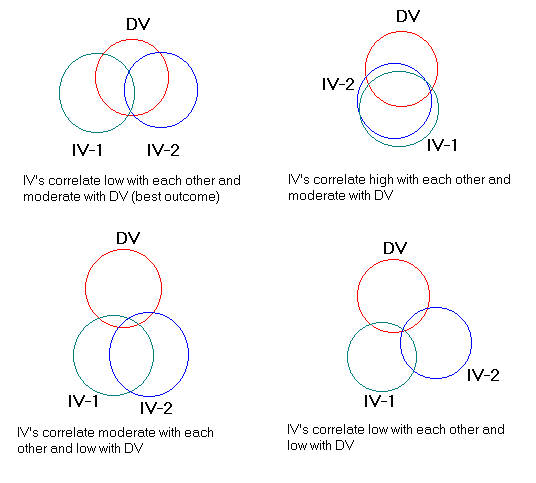
In the first run Tense accounted for 12% variance beyond Anger and in the second run Anger accounted for 7% variance beyond Tense. These two runs are represented in the Venn diagram below. These percentages can be shown in a Venn diagram. Overlaps of variables indicate shared variance. For example, in the figure below there is 12% overlap between the X-1 variable and the Y variable.
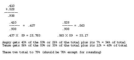
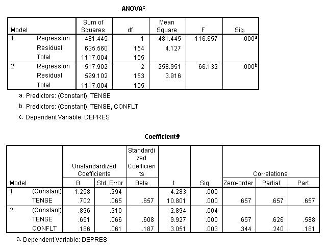
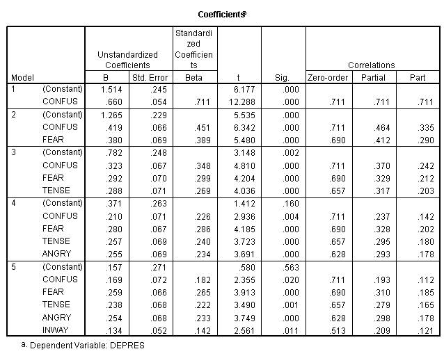
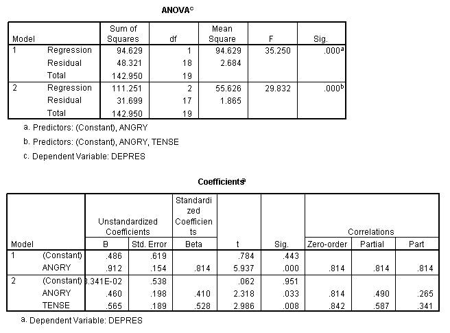
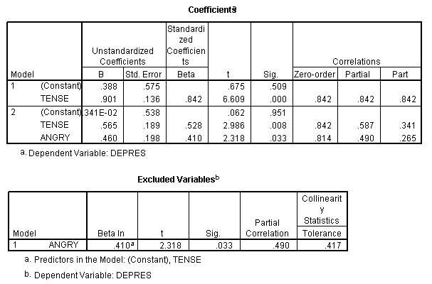
It appears that it makes no difference whether you think about the beta weight as being taken directly from the part correlation or whether you take the part correlations plus the respective amount of weight from the overlap -- the proportional weight is the same.